# A tibble: 7 × 7
  person_ID household_ID gender   age income neighborhood_income
      <int>        <dbl> <chr>  <dbl>  <dbl> <chr>
1         1            1 f         31   1039 low income
2         2            1 f         30   1677 low income
3         3            2 m         45   4971 low income
4         4            3 m         42   3274 high income
5         5            4 m         32   3937 high income
6         6            6 f         42   2031 high income
7         7            7 f         46   3463 high income
# ℹ 1 more variable: n_people_household <dbl>Tidyverse
Introduction
Packages
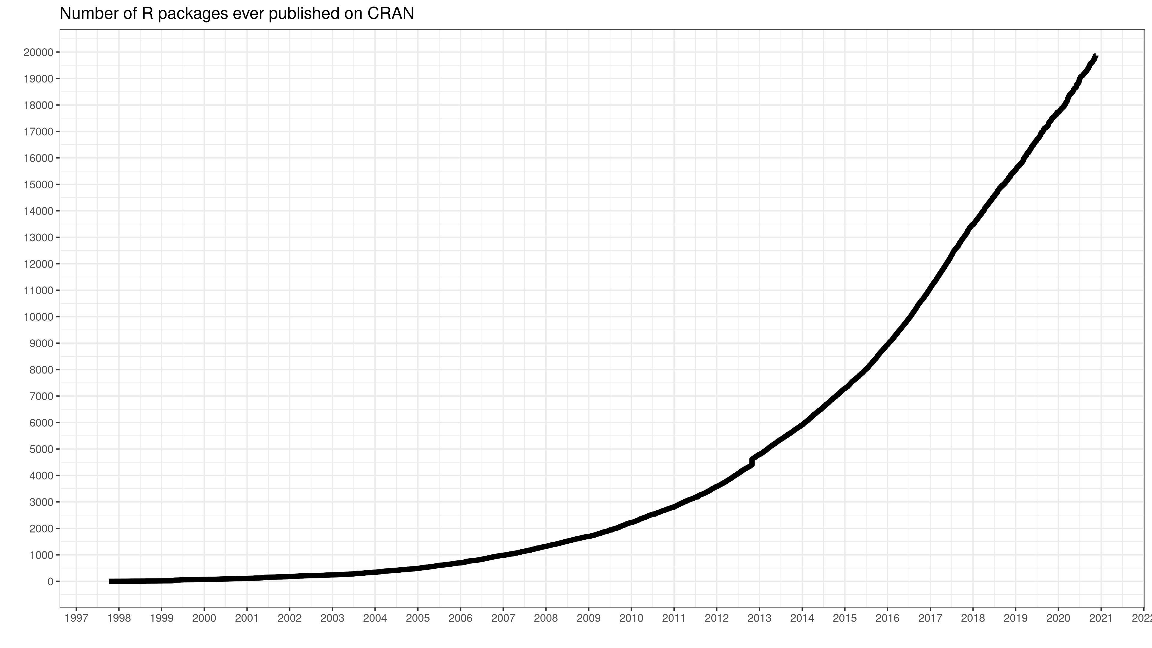
One of the main advantages that R has as a software for statistic analysis is its incremental syntax. This means that the things you can do in R are constantly updated and expanded through the creation of new packages, developed by researchers, users or private companies.
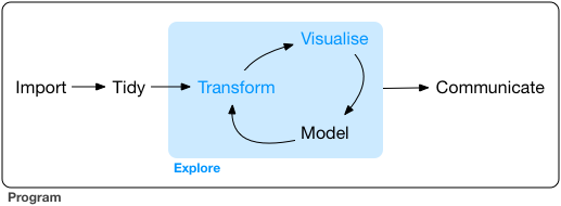
These packages contain code, data, and documentation in a standardized collection that can be installed by users of R. Most of the time, we will install them in order to use functions that will do certain tasks that help us work with our data. So far, we were using functions contained in R base: such as mean(), median(), quantile(), etc. But as we dive deep into the data science life cycle, we might address certain challenges that require more complex, or specific, functions. We will need to import the data, tidy the data into a format that is easy to work with, explore the data, generate visualizations, carry out the analysis and communicate the insights. The tidyverse ecosystem provides a powerful tool for streamlining the workflow in a coherent manner that can be easily connected with other data science tools.
tidyverse + Data workflow
The tidyverse is a set of R packages designed for data science. The main idea behind tidyverse is to contain in a single installation line, a set of tools that contain the entire data analysis workflow: from the importation of data to the communication of results.
Tidy data
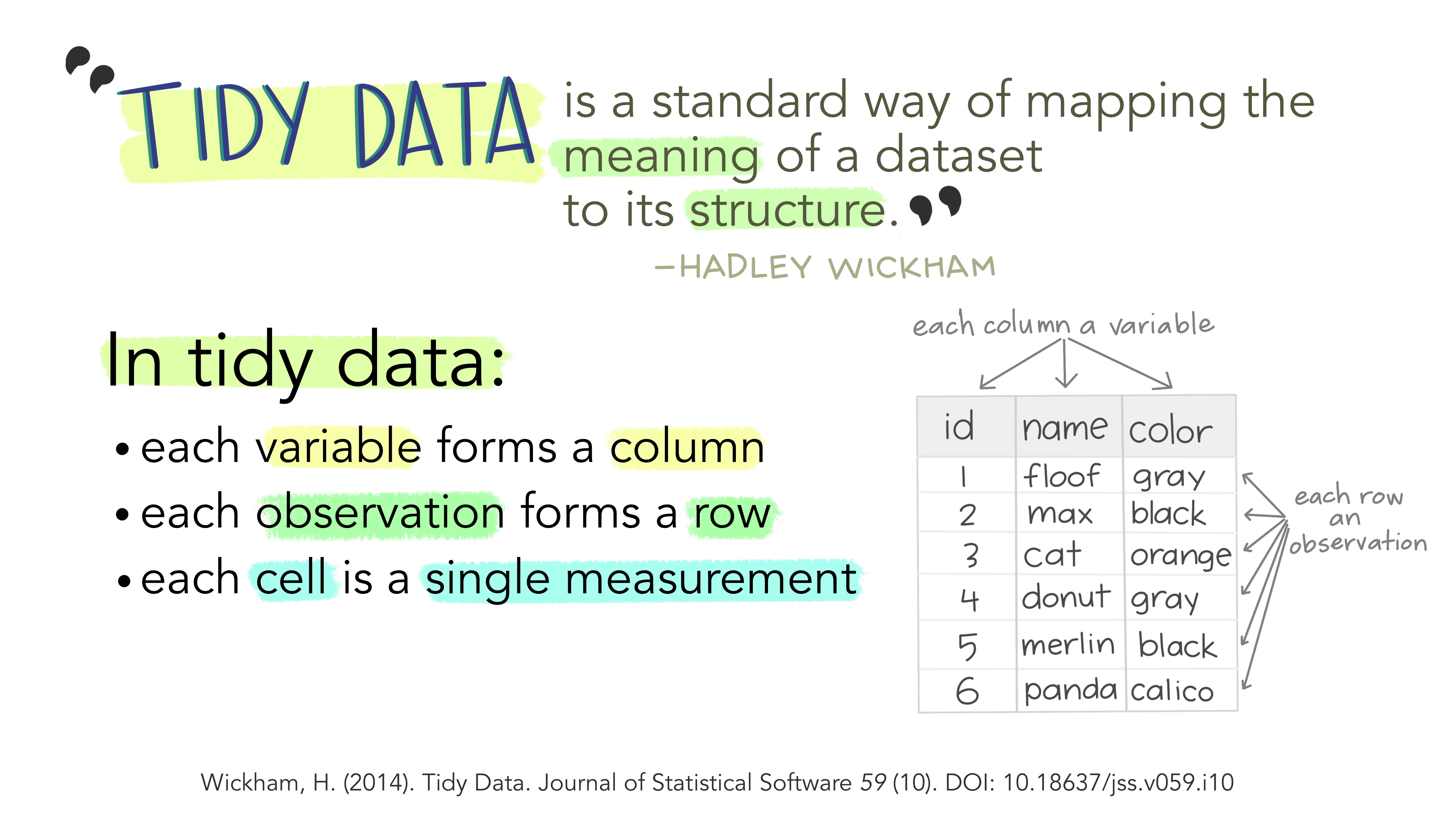
All packages share an underlying design philosophy, grammar, and data structures. These structures refer to the format of tidy datasets. But, what is tidy data? It is a way to describe data that’s organized with a particular structure: a rectangular structure, where each variable has its own column and each observation has its own row (Wickham 2014a; Peng n.d.).
According to (Wickham 2014b),
“Tidy datasets are easy to manipulate, model and visualize, and have a specific structure: each variable is a column, each observation is a row, and each type of observational unit is a table.”
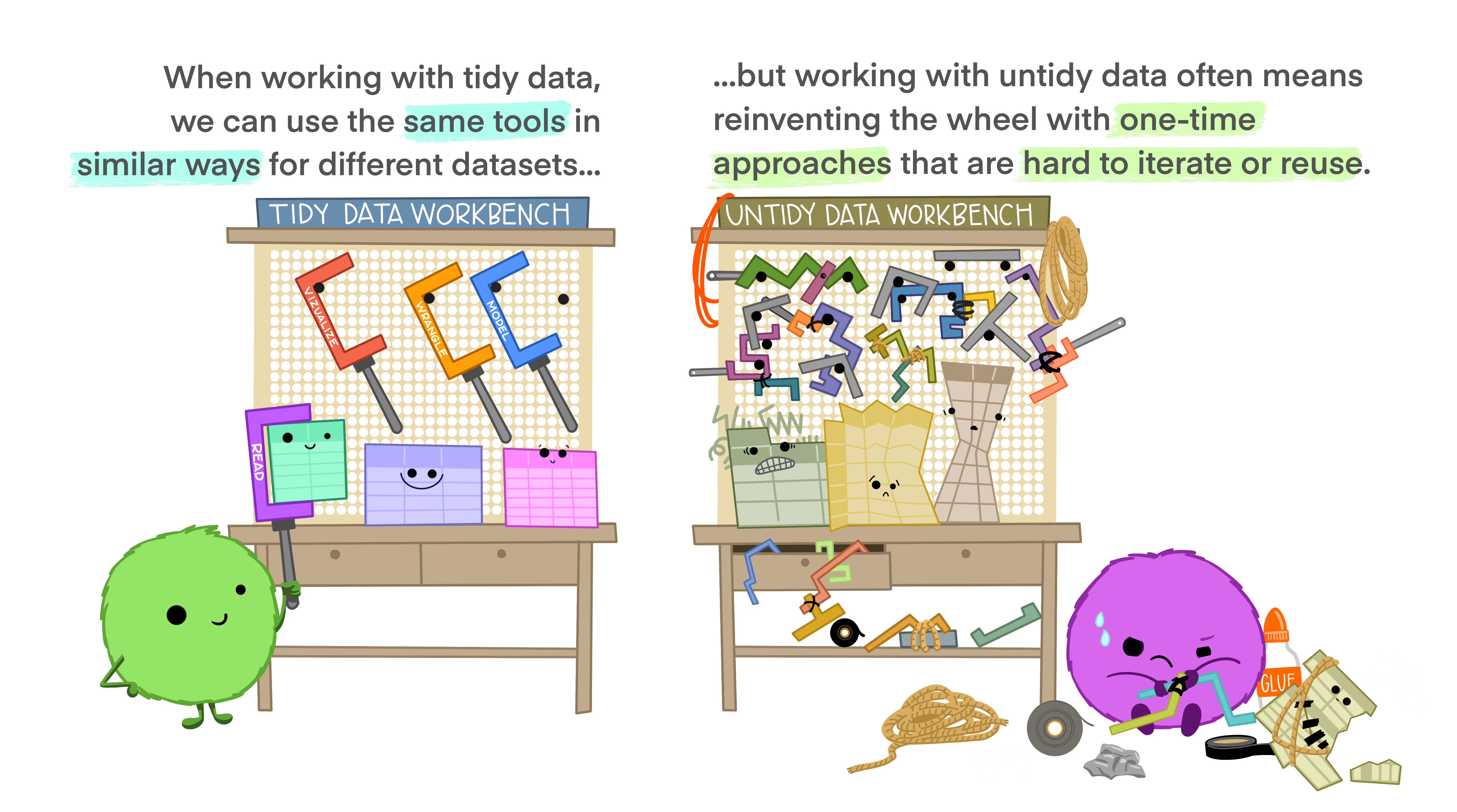
Working with tidy data means that we work with information that has a consistent data structure. The main benefit behind this is that we will have to spend less time thinking how to process and clean data, because we can use existing tools instead of starting from scratch each time we work with a new dataset. In other words, we only require a small set of tools to be learned, since we can reuse them from one project to the other.
tidyverse ecosystem
We can think of the tidyverse ecosystem (Grolemund n.d.) as the set of tools we can reuse in our tidy data. It is an ecosystem because consists in a set of various packages that can be installed in one line of code (install.packages(tidyverse)), and each package fits into a part of the data science life cycle. This is the main reason why we prefer to use tidyverse instead of R base. It provides us with a consistent set of tools we can use for many different datasets, it is designed to keep our data tidy, and it contains all the specific tools we might need in our data science workflow.
There is a set of core tidyverse packages that are installed with the main ecosystem, which are ones you are likely to use in everyday data analyses.
tibble: it is a package that re-imagines the familiar R data.frame. It is a way to store information in columns and rows, but does so in a way that addresses problems earlier in the pipeline. That is to say, it stores it in the tidy data format. The official documentation calls tibbles ‘lazy and slurly’, since they do less (they don’t change variable names or types, and don’t do partial matching) and complain more (e.g. when a variable does not exist). This forces you to confront problems earlier, typically leading to cleaner, more expressive code.readr: this is a package we will use every time we start a new project. It helps read rectangular data into R, and it includes data in .csv and .tsv format. It is designed to flexibly parse many types of data found.- to read data in .xlsx or .xlx format, you should install the tidyverse-adjacent package
readxl.
- to read data in .xlsx or .xlx format, you should install the tidyverse-adjacent package
dplyr:designed for data wrangling. It is built around five primary verbs (mutate, select, filter, summarize, and arrange) that help make the data wrangling process simpler.tidyr:it is quite similar todplyr, but its main goal is to provide a set of functions to help us convert dataframes into tidy data.purr:enhances R’s functional programming toolkit by providing a complete and consistent set of tools for working with functions and vectors. It makes easier for us to work with loops inside a dataframe.stringr:it is designed to help us work with data in string format.forcats:it provides functions to help us work with data in the factor format.ggplot:the main package for data visualization in the R community. It is a system for declaratively creating graphics, based on The Grammar of Graphics. You provide the data, tell ggplot2 how to map variables to aesthetics, what graphical primitives to use, and it takes care of the details.
While this is the main structure of the tidyverse ecosystem, there are multiple adjacent packages that we can install which fit into the tidy syntax and work well with the tidy data format. Some of them are readxl to read data in .xlsx or .xl format, janitor for cleaning data, patchwork to paste ggplot graphs together, tidymodels for machine learning… and many more.
Tidy data functions
As you had a glimpse in the previous classes, there are some basic functions that we use to tidy data:
mutate: to transform columnsselect: to select certain columnsfilter: to select certain rows (we can think of filter as the row-wise version of select, and select as the column-wise version of filter)arrange: to reorder values of rows
Now, we will go over the basics of more complex data transformation functions to reshape the data: joins, pivots, summarizes and date processing.
Merges of dataframes
If you ever worked with SQL or multiple databases in the past, you might already be familiar with the concept of joining data. A tidy dataset should contain one type of observational unit per table. For example, if we have done a survey regarding labor conditions to individuals, but we also have sociodemographical information regarding their household, we should have each information in a different dataset. However, we will probably be interested in crossing the information regarding the individuals and their household conditions. So we need to have key IDs to be able to combine these two datasets: for example, in this case, the ID for the household.
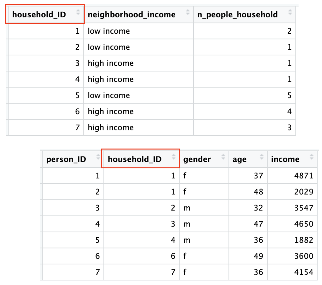
Note that the household ID is not the same as the person ID. Each person has a unique identifier, but so does each household. The information is consistent: when we have two individuals who share a household ID, we see in the household information that there are two people living there.
Now, how do dataframe joins work?
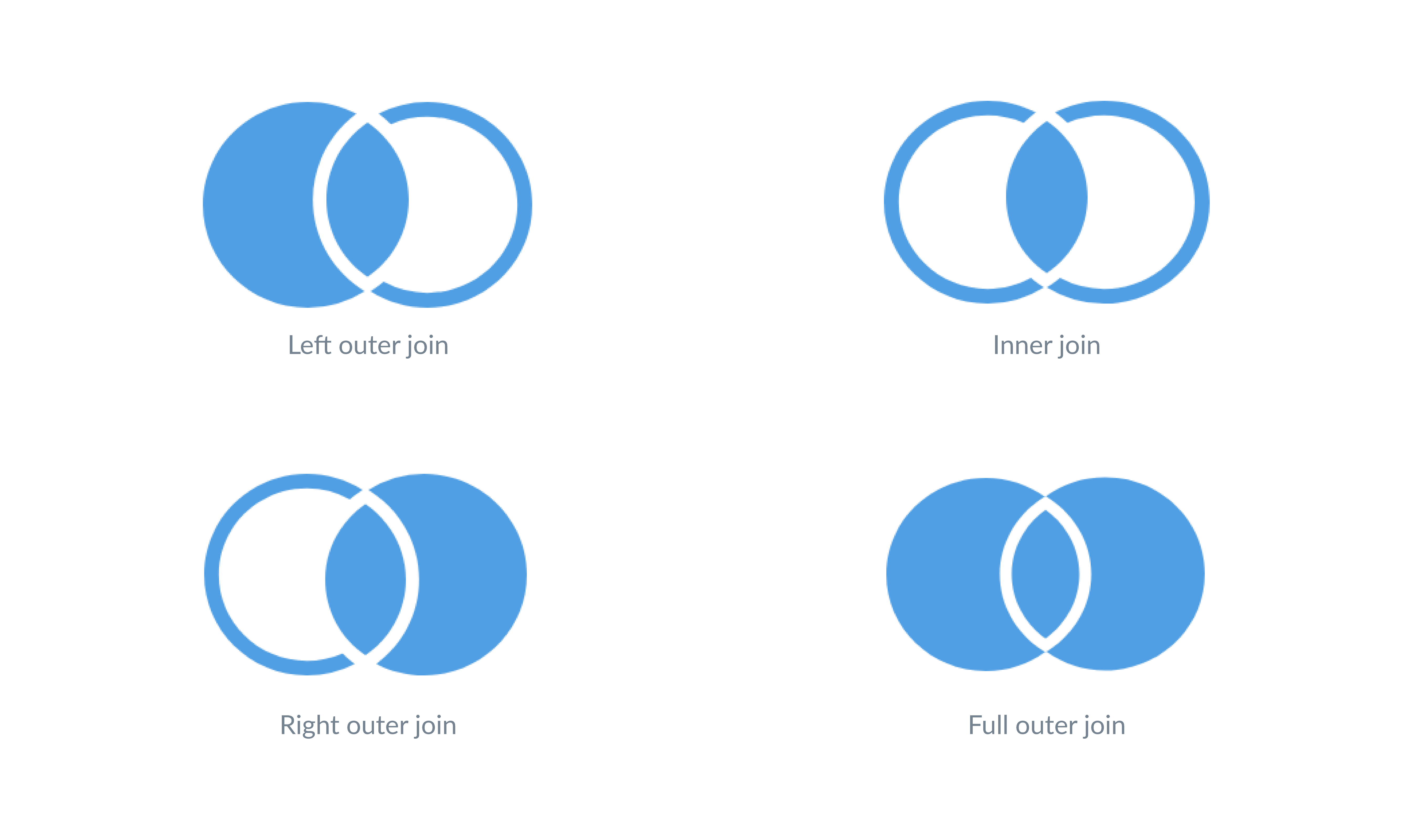
- Inner join: this creates a new dataset that only contains the information of rows where the IDs match. For example, in our case, the data of the household 5 wouldn’t appear since it doesn’t join any individual data.
- Left join: it keeps all the rows of the data on the “left” and adds the columns that match the dataframe on the right. The decision of which dataframe goes where (left or right) is arbitrary and up to us, but we must keep in mind that it will be our main dataframe in the join. In our example, if we chose the individual dataset as the left, we would have the same table as the result of the inner join. But if we chose the household dataset, we would have a dataset with empty values for the ID’s that don’t match.
# A tibble: 8 × 7
  household_ID neighborhood_income n_people_household person_ID gender   age
         <dbl> <chr>                            <dbl>     <int> <chr>  <dbl>
1            1 low income                           2         1 f         31
2            1 low income                           2         2 f         30
3            2 low income                           1         3 m         45
4            3 high income                          1         4 m         42
5            4 high income                          1         5 m         32
6            5 low income                           5        NA <NA>      NA
7            6 high income                          4         6 f         42
8            7 high income                          3         7 f         46
# ℹ 1 more variable: income <dbl>- Full join: it keeps all the columns and all the rows in both dataframes.
# A tibble: 8 × 7
  household_ID neighborhood_income n_people_household person_ID gender   age
         <dbl> <chr>                            <dbl>     <int> <chr>  <dbl>
1            1 low income                           2         1 f         31
2            1 low income                           2         2 f         30
3            2 low income                           1         3 m         45
4            3 high income                          1         4 m         42
5            4 high income                          1         5 m         32
6            5 low income                           5        NA <NA>      NA
7            6 high income                          4         6 f         42
8            7 high income                          3         7 f         46
# ℹ 1 more variable: income <dbl>
Summarizing information
Many times, we will want to summarize the information in our dataset. We can catch a glimpse of the summarized dataset with functions such as summary() or str(). However, more often, we will want to see specific information regarding groups in our dataset. For example, how many households we have in the different types of neighborhoods. To do this, it is necessary to group our data. We will not look into the total number of households, but we will group the data by the neighborhood of the households. Then, we can count each group.
# A tibble: 2 × 2
  neighborhood_income     n
  <chr>               <int>
1 high income             4
2 low income              3
Other times, we might be interested in getting descriptive statistics per group. For example, the median age for men and women in the individuals dataset.
# A tibble: 2 × 2
  gender median_age
  <chr>       <dbl>
1 f            36.5
2 m            42
Or even combine groups and subgroups. For example, the median income for women and men who live in low income or high income neighborhoods
# A tibble: 4 × 3
# Groups:   neighborhood_income [2]
  neighborhood_income gender income
  <chr>               <chr>   <dbl>
1 high income         f       2747
2 high income         m       3606.
3 low income          f       1358
4 low income          m       4971
Reshaping data
Converting your data from wide-to-long or from long-to-wide data formats is referred to as reshaping your data.
For example, take this subset of columns from our individuals dataset.
# A tibble: 7 × 4
  person_ID gender   age income
      <int> <chr>  <dbl>  <dbl>
1         1 f         31   1039
2         2 f         30   1677
3         3 m         45   4971
4         4 m         42   3274
5         5 m         32   3937
6         6 f         42   2031
7         7 f         46   3463
This is what we call a wide format: each variable has its own column, and each row represents a single observation. Long data, on the other hand, refers to a dataset where each variable is contained in its own column. This format is often used when working with large datasets or when performing statistical analyses that require data to be presented in a more condensed format.
This is the same dataset we had previously but reshaped as long data.
# A tibble: 14 × 4
   person_ID gender variable value
       <int> <chr>  <chr>    <dbl>
 1         1 f      age         31
 2         1 f      income    1039
 3         2 f      age         30
 4         2 f      income    1677
 5         3 m      age         45
 6         3 m      income    4971
 7         4 m      age         42
 8         4 m      income    3274
 9         5 m      age         32
10         5 m      income    3937
11         6 f      age         42
12         6 f      income    2031
13         7 f      age         46
14         7 f      income    3463
As you can see, the wide data format has a separate column for each variable, whereas the long data format has a single “variable” column that indicates whether the value refers to age or income.
Dates in R
Dates are a special type of object in R. There are three types of data that refer to an instant in time:
A date. Tibbles will print it as
date.A time within a day. Tibbles will print it as
time.A date-time, which refer to dates plus times, specifying an exact moment in time. Tibbles print this as
<dttm>. In R base, these are called POSIXct.
It is a good practice to keep our data simple, so if we don’t necessarily need the time information to work in our project, we will usually prefer to work with date formats.
When working with dates in R, we should also be careful with time zones. Time zones are an enormously complicated topic because of their interaction with geopolitical entities. R uses the international standard IANA time zones. You can find out what R thinks your time zone is using the following command:
Sys.timezone()[1] "America/Toronto"lubridate uses UTC (Coordinated Universal Time), which is the standardized time zone used by the scientific community.
Discussion
During this class, we went over the tidyverse functions that we use for preprocessing and transforming the data. This is a crucial step of the data science workflow. Most of the times, we will receive a non-tidy dataset with many errors (NA’s, wrong formats in columns…) and a large portion of our work will be dedicated to tidying the data. Then, this will be the raw material we use to make our analysis and communicate the results. This is why it is a huge, important step in the workflow, not only because of technical difficulties, but also some conceptual problems might emerge.
Another problem can show up in the merging of databases. We should be careful to not join data just because they share and ID or a value (for example, a city or a state). Datasets are only comparable when the population of reference is the same in both. So, if we join two tables that don’t share a population, we should explicit so and explain why we are doing it. For example, are we using it as a control variable? How different are the populations?
In this sense, this is why it is important to keep a record of the code we use for preprocessing the data. The analysts’ bias can be introduced during this process, so it is important to keep track of this in order to guarantee reproducibility and to be held accountable of our methodological decisions.
