Evaluation
Introduction
So far, we addressed different statistical and machine learning methods we can use to predict different values in datasets. Why is it necessary to introduce so many approaches, instead of just one? In statistics, there is no ideal universal approach for every dataset and problem. The results will vary depending on the approach, the research questions and the data, and in return it is important to decide for any given set of data which methods produce the best results. The definition of ‘best result’ is also not universal, because it depends on our goal with the predictions. Broadly speaking, are we interested in capturing as many cases as possible? Or are we interested in capturing specific, correct cases?
In this class we will address different ways to measure how ‘fit’ our model is given our dataset and project goals.
Evaluating model data
In order to evaluate the performance of a predictive method on a given data set, we need some way to measure how well its predictions actually match the observed data. It is necessary to quantify the extent to which the predicted response value for a given observation is close to the true response value for that observation. This can easily be done comparing the real results and the predicted results.
However, what do you think about comparing the real values and the predictions, when these are product of a model fitted and trained over the same dataset?
It is likely that (unless our model is very, very bad) the predictions will match the real values almost perfectly. This is because the model has learned through the observations and knows how the target behaves with the specific different combinations of features. However, we are also interested in knowing how well the method will perform on new, unseen data with new features. If we only focus on the results of the model on the trained dataset, this can likely lead to a phenomenon called overfitting. This is how we refer to the situation where a model adapts too much to the training data; it performs well for the data used to build the model but poorly for new data (Silge and Julia, n.d.).
Overfitting: In colloquial terms, it’s as if the model learns the relationship between the predictive variables and the variable to be predicted by heart, and this leads it to be unable to answer new questions that were not asked before.
How can we evaluate the model’s performance on new data if we only have our original dataset? We will explore various approaches to this in the course.
Validation set approach
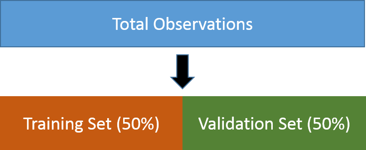
The validation set approach, also known as “hold-out validation” or “simple validation,” is a straightforward technique used to evaluate models. It entails randomly dividing the available observations into two parts: a training set and a validation set. The model is trained on the training set, and then used to predict responses for the observations in the validation set. The resulting validation set error rate serves as an estimate of the test error rate.
Typically, a random partition allocates a substantial proportion of the dataset, usually around 70% to 80%, to the training set. This segment serves as the foundation for model development, where the model is fitted and trained. The remaining observations form a distinct validation set, enabling us to gauge the model’s performance on previously unseen data. Results from the validation set provide insights into how the model may perform with new, unencountered data, as these observations were excluded from the model’s learning process, allowing us to assess its generalization capabilities.
In most cases, we employ random sampling to divide the data into the train/validation set. However, situations may arise where the classes in the data are imbalanced. An imbalanced dataset occurs when one class constitutes a significant portion of the training data (the majority class), while the other class is underrepresented (the minority class). This imbalance can lead to bias in our model, causing it to favor one class over the other. Consequently, the model may exhibit strong performance on the training data but struggle with new data. To address this issue, we can consider three strategies to balance the data.
Capturing more cases: To address imbalanced datasets, researchers have several options. One approach involves capturing more cases to achieve a balanced sample. Alternatively, data augmentation techniques can be employed. Data augmentation involves expanding our sample by applying various transformations to the existing data. For structured data, this may include introducing synthetic noise or generating new samples by perturbing existing data points. Techniques such as adding random values or utilizing statistical methods can be used for this purpose.
Subsampling the data: It involves reducing the size of the majority class until it occurs with the same frequency as the minority class. This approach typically results in better-calibrated models, where the distributions of class probabilities are more consistent. Another method is oversampling, where the sample of the minority class is increased to match the frequency of the majority class through resampling1 (“Tidymodels - Subsampling for Class Imbalances,” n.d.). However, oversampling may lead the model to memorize training data patterns, especially when the minority class consists of a limited number of unique data points, potentially causing performance issues on the validation set.
Cross-validation
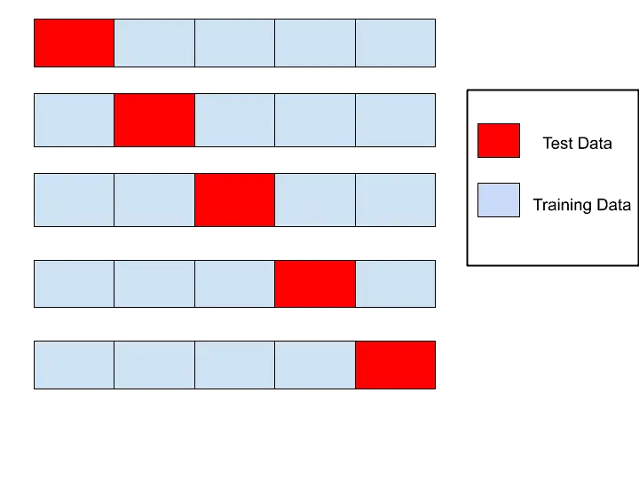
Cross-validation is a method that entails randomly dividing the observation dataset into k groups or “folds,” each approximately equal in size. During each iteration, one fold is designated as the validation set, while the model is trained on the remaining k-1 folds. This process repeats k times, with each iteration utilizing a different fold as the test set and the remaining folds as the training set.
K-fold cross-validation offers several advantages:
Robust Performance Estimate: By testing the model on different subsets of the data, it provides a more robust estimate of its performance. This is essential for evaluating how well the model generalizes to unseen data.
Overfitting Detection: It helps in detecting overfitting by testing the model on multiple diverse data subsets, unlike the validation set approach, which uses only one subset.
Optimal Use of Data: It maximizes the utilization of available data for both training and testing purposes, particularly beneficial when dealing with limited data resources.
Bias variance trade-off
These approaches for evaluating a model’s performance on new data are crucial for experimenting with different hyperparameters and predictive methods to determine the best fit for a particular use case. They help in defining whether our data is better predicted with a more flexible or simpler, rigid model. Additionally, they allow us to identify two sources of error that affect a model’s performance: bias and variance. (Johnson and Kjell, n.d.).
- Bias refers to the error introduced by approximating a complex real-life problem with a much simpler model. For instance, using linear regression to analyze intricate social issues like hours dedicated to domestic work may lead to bias because linear regression is overly simplistic and may not capture underlying data patterns. This situation is known as underfitting, where the model fails to generalize well to the data.
- Variance, on the other hand, refers to the opposite scenario. It arises when large, complex models exhibit significant changes with variations in the training data. This is characteristic of overfitting, where the model performs exceptionally well on the training dataset but struggles with new, unseen data.
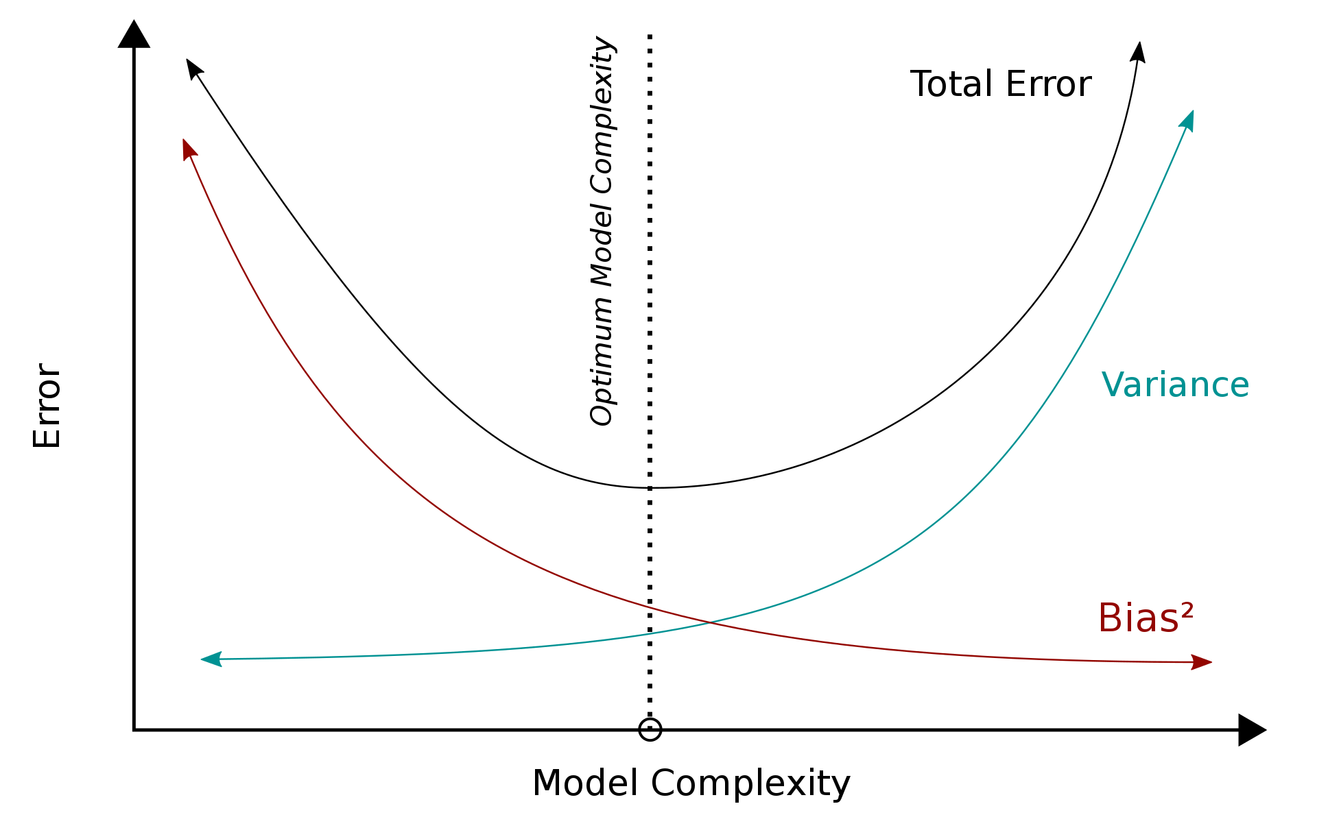
In practice, there’s often a trade-off between these two types of errors. Simple models typically show high bias and low variance, while complex models tend to have low bias but high variance. Therefore, during the processes of training, fine-tuning, and evaluating a method, our objective is to pinpoint the optimal level of model complexity that strikes a balance, minimizing both bias and variance. This equilibrium ensures that the model can effectively capture underlying data patterns while still generalizing well to new data.
The figure illustrates how a model’s complexity impacts the generalization error. As the model becomes more complex, the variance tends to increase while the bias decreases. Eventually, there’s a point where the bias and variance intersect, leading to the lowest generalization error, or the lowest error rate for the test set. This point represents the optimal balance of bias and variance for the given problem, where the bias-variance trade-off is minimized.
Metrics for Evaluation
After training our data and making predictions on a new dataset, evaluating the effectiveness of the model becomes essential. It’s crucial to recognize that the definition of an effective model varies depending on its intended use.
Depending on the purpose, models can be broadly categorized into inferential and predictive models, with each prioritizing different aspects of modeling.
Inferential Models: These models are primarily utilized to comprehend relationships within the data, with a significant emphasis on selecting and validating probabilistic distributions and other generative characteristics. The main objective is to gain insights into the underlying processes driving the observed data, prioritizing the validity and interpretability of the models. In essence, inferential models aim to offer a meaningful understanding of how variables are related and to draw inferences about the population from which the data originated.
Predictive Models: In contrast, predictive models are chiefly intended for making accurate predictions, focusing primarily on the model’s capability to provide reliable and precise predictions of future or unseen data. The primary measure of success for predictive models lies in how closely their predictions match actual observations. Essentially, predictive strength is determined by the model’s consistency in providing accurate predictions, with lesser emphasis on the underlying statistical qualities if the model consistently delivers accurate predictions. A quantitative approach to estimating effectiveness enables us to comprehend, compare, and enhance models’ performance.
In this course, we will focus on effectiveness measures for predictive models. Quantifying the model’s performance through metrics enables us to comprehend, compare, and enhance its performance. Various metrics exist to gauge how well our model performs for different types of variables, whether numeric or categorical.
Metrics for regression
In supervised learning, when our objective is to forecast a continuous numeric value, we encounter regression problems. Some examples include:
Predicting a persons’ income based on their work experience, age, gender, race, years of education.
Estimating the potential sales of a product.
Projecting the graduation rate of students in schools across different neighborhoods.
Predicting GDP per capita in various countries, considering developmental variables.
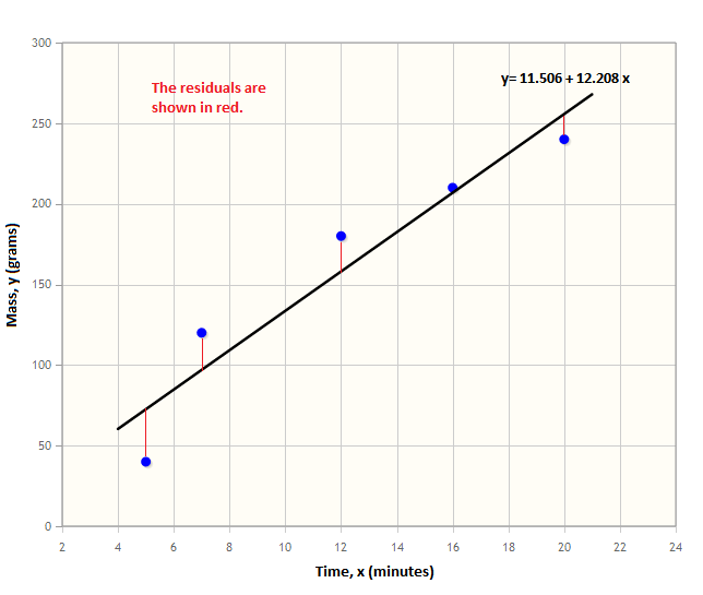
Intuitively, one of the simplest methods to evaluate the effectiveness of a model’s predictions is by calculating the difference between the predicted values and the actual values. This difference, often termed the residual, is computed for each observation.
The Mean Absolute Error (MAE) calculates the average of these residuals within the model, providing insight into the magnitude of the deviations between predictions and actual outputs. However, MAE does not indicate the direction of the errors, such as whether the model underestimates or overestimates the data. Its formula is:
\[ \sum_{i=1}^{D}|x_i-y_i| \]
Where \(|x_i-y_i|\) represents the absolute difference between the \(i\)-th observed value \(y_i\) and the \(i\)th predicted value (\(x_i\)).
In machine learning, a common variation of MAE is Mean Squared Error (MSE). MSE computes the average of the squared differences between the actual values and the predicted values. The primary advantage of MSE is its capability to amplify the impact of larger errors by squaring the differences, thereby emphasizing significant deviations more prominently. This property makes MSE particularly effective in highlighting and pinpointing substantial disparities between predictions and actual outcomes. The MSE is given by:
\[ sum_{i=1}^{D}(x_i-y_i)^2 \]
Metrics like these allow us to assess the accuracy of a model. Accuracy, in the context of machine learning, quantifies the proportion of correct predictions made by a model relative to the total number of predictions.
In contrast, a metric such as the coefficient of determination (also known as \(R^2\)) enables us to measure the correlation between the dependent variable and the independent variables. This value offers insights into the model’s capacity to explain the predictions of the target variables and is calculated using the following formula:
\[ 1−∑(yi−yi)^2/∑(yi−y)^2 \]
This coefficient produces a score between 0 and 1, where a value closer to 1 signifies better performance of the model.
Metrics for classification
Classification problems involve predicting the output of a categorical variable. Examples include:
Predicting employment status of a person.
Predicting highest level of education achieved.
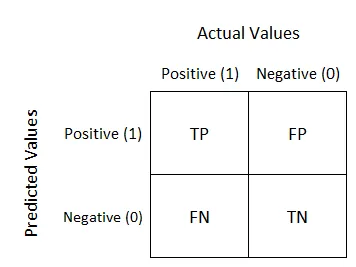
When evaluating a classification model, a common approach is to compare the observed category with the predicted category. These comparisons can be visualized using a confusion matrix:
There are four possible outcomes in the result of a classification:
True Positives (TP): Observations belonging to the positive class and correctly classified as such by the model. The model accurately identifies cases that are genuinely positive.
False Negatives (FN) or Type I error: Observations that actually belong to the positive class but are incorrectly classified as negative by the model. In this case, the model fails to identify instances that are genuinely positive.
True Negatives (TN): Observations belonging to the negative class and correctly classified as such by the model. The model correctly identifies cases that are genuinely negative.
False Positives (FP) or Type II error: Observations that actually belong to the negative class but are incorrectly classified as positive by the model. In this scenario, the model mistakenly identifies instances as positive when they are genuinely negative.
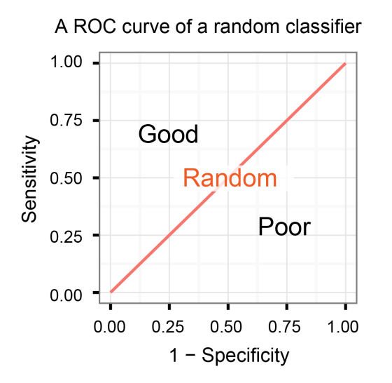
These outcomes provide ways to evaluate the model. One common method is using the Receiver Operating Characteristic (ROC) curve. The ROC curve is a graphical representation of a model’s performance, showing the trade-off between the true positive rate (TPR: the model’s ability to correctly identify positive cases) and the false positive rate (FPR: the model’s tendency to classify negative cases as positive) across different thresholds.
The ROC space is defined by placing the TPR or sensitivity in the y-axis, and the FPR in the x-axis. Given different thresholds for classifying an observation into a positive class, different values for these two rates are achieved. The ROC curve illustrates all these points graphically, typically starting at the bottom-left corner (0,0) and ending at the top-right corner (1,1).
An ideal ROC curve would hug the top-left corner of the graph, indicating a model that achieves high true positive rates while keeping false positive rates low across all thresholds. In contrast, a diagonal line from the bottom-left to the top-right corner represents a model with no predictive ability, where the true positive and false positive rates are roughly equal.
The area under the ROC curve (AUC-ROC) is often used as a single metric to summarize the model’s overall performance. A higher AUC-ROC value (closer to 1) indicates better discrimination between positive and negative cases by the model.
We utilize different metrics to evaluate the performance of our model based on the specific goal of the prediction. If our aim is to identify the maximum number of relevant cases, we prioritize recall as our metric for assessing results. Conversely, if our focus is on pinpointing true positives with the highest accuracy, precision becomes the chosen metric, emphasizing the precision of true positive predictions. The choice of metric depends on the context and the specific objectives of the analysis.
Precision: It is a measure of the accuracy of positive predictions made by the model. It quantifies the proportion of positively labeled instances predicted by the model that are actually correct. High precision indicates that when the model predicts a positive instance, it is more likely to be correct.
Precision is calculated as the ratio of true positives (correctly predicted positive instances) to the sum of true positives and false positives (instances predicted as positive but are actually negative). It is given by the formula:
\[ TP/(TP + FP) \]
Recall: Also known as Sensitivity or True Positive Rate (TPR), measures how many of the actual positive instances were correctly predicted by the model. High recall indicates that the model effectively captures most of the positive instances.
Recall is calculated as the ratio of true positives to the sum of true positives and false negatives (instances that are actually positive but were predicted as negative). It is given by the formula:
\[ TP / (TP + FN) \]
F1 Score: providing a balanced measure between these two metrics. It is particularly useful when you want to consider both precision and recall simultaneously, ensuring a balance between false positives and false negatives. This metric is especially valuable in scenarios with imbalanced datasets, where one class significantly outnumbers the other. The F1 Score is calculated using the formula:
\[ 2*(Precision*Recall)/(Precision + Recall) \]
Discussion
Let’s exemplify the latter with a practical scenario. In the realm of public administration, machine learning emerges as a valuable tool for identifying vulnerable populations and effectively allocating resources to support them. Imagine you’re a government data scientist tasked with constructing a model to predict individuals at risk of eviction. The overarching aim is to recognize these individuals and provide them with financial assistance to prevent homelessness. Following the principles we’ve acquired thus far, we would embark on developing a model, training it with various hyperparameters using a portion of the dataset, and assessing its performance on the remaining data points.
Upon evaluating several models, we observe a trade-off: models with higher recall exhibit lower precision, while those with lower recall demonstrate higher precision. So, which option is optimal? In this scenario, particularly when our focus is on leveraging machine learning to aid vulnerable populations, we would favor prioritizing higher recall. While such a model might misclassify some individuals at risk of eviction, it’s crucial to recognize that vulnerability often extends across multiple dimensions. Indeed, excessively fixating on the precision and accuracy of the classification model could potentially hinder our overarching objective of reducing inequality within the population.
Addressing inequalities necessitates a willingness to accept a notable decrease in accuracy or the development of innovative, sophisticated methodologies to foster more practical approaches to reducing disparities in such applications (Rodolfa, Lamba, and Ghani 2021).
References
Footnotes
Resampling implies repeating cases to get the desired n.↩︎
